【python】有限要素法(FEM)をゼロから実装する6_応力のカラーマップ作製

はじめに

これまで静弾性問題の有限要素解析の実装を進めてきました。これまでの記事で変形まで求めることはできましたが、なんだか以下の結果だと見栄えが物足りないですよね。

FEMといえばよく見るのは上記のグラフを応力の値に応じて色を塗るカラフルな応力プロットだと思うのでそれの実装まで行いたいと思います。

はじめに
応力の算出
応力のカラーマップ
- 実装
コード
終わりに
参考文献

応力の算出

応力とひずみの関係式

節点の変位まで求まったので、応力とひずみの関係式より応力を求めることができます。
過去の記事で関係式の整理をしましたが、応力とひずみの関係式は以下の形になります。

$\boldsymbol{\sigma} = \boldsymbol{DBd_{e}}$

ここで $\boldsymbol{d_{e}}$ は要素の各節点の変位をまとめた節点変位ベクトルであり、各ノードの変位( $(x, y)$ 座標系)を $(u_{i}, v_{i})$ とすると以下です。
つまり要素ごとにこの式を解いて、各要素の応力を求める必要があります。

$\boldsymbol{d_{e}} = \begin{bmatrix} u_{1} \\ v_{1} \\ u_{2} \\ v_{2} \\ u_{3} \\ v_{3} \\ u_{4} \\ v_{4} \\ \end{bmatrix}$

$\boldsymbol{B}$ は $(\xi, \eta)$ の関数であり、要素剛性マトリクスを求めた際は積分点でのBマトリクスを導出していたので今回も積分点を代入します。つまり、上記の応力とひずみの関係式で求められる $\boldsymbol{\sigma}$ は要素内の積分点における応力を表します。

応力をプロットするうえで、節点における応力を求めたいので次に節点応力の求め方について解説します。

節点応力の導出

各要素の各積分点での応力から近似的に節点応力を求める方法はいくつかあるみたいですが、基本的には以下の2ステップで実装します。

要素内の各積分点での応力とその平均応力から要素ごとに各節点の応力を外挿して求める
各節点を共有する要素ごとにその節点での外挿値が求まるのでそれを平均してその節点の応力とする

要素ごとに各節点の応力を外挿する

外挿の仕方は、今回一番簡単かつよく使われる線形外挿法を用います。
要素の中心から各積分点までの距離と節点までの距離の比は $\sqrt{3}$ なので以下のようにそれぞれの節点の外挿値を求めます。

(要素における節点1の外挿値) = (要素の平均応力)+{(節点1に一番近い積分点での応力)-(要素の平均応力)} * $\sqrt{3}$

節点の応力の外挿値を節点を共有する要素間で平均する

これはそのまま平均するだけです。
例えば要素1と2のみが節点1を共有している場合、要素１、要素２それぞれで節点1の応力外挿値が求まるのでそれらを平均すればOKです。

節点応力の計算の実装

では上記のことを踏まえて実際に実装してみます。
Solverクラスに応力計算用の関数を作ってそこで実装します。

class Solver:
    """
    有限要素法の計算を行うクラス
    
    Attributes:
        mesh (Mesh): Meshクラス
        material (Material): Materialクラス
        D (array 3x3): Dマトリクス
    """
##########略################
    
    def calc_stress(self):
        """
        節点応力を算出。

        Args:
            elem (Element): 対象のElementクラス

        Returns:
            stress_e (array 3x1): 節点応力
        """
        stress_dict = {i : np.zeros(3) for i in range(len(self.mesh.nodes))}
        counts_dict = {i : 0 for i in range(len(self.mesh.nodes))}

        gps = ((-1 / np.sqrt(3), -1 / np.sqrt(3), 1, 1), 
              (1 / np.sqrt(3), -1 / np.sqrt(3), 1, 1), 
              (1 / np.sqrt(3), 1 / np.sqrt(3), 1, 1), 
              (-1 / np.sqrt(3), 1 / np.sqrt(3), 1, 1), 
              )
        
        for elem in self.mesh.elements:
            nodes_ind = []
            for ind in elem.node:
                nodes_ind.append(ind * 2)
                nodes_ind.append(ind * 2 + 1)
                d_elem = self.d[nodes_ind]

            stress_e = {}
            ave_stress_e = np.zeros(3)
            for i, gp in enumerate(gps):
                xi, eta = gp[0], gp[1]
                B, J = self.calc_B(elem, xi, eta)
                stress_e[i] = np.dot(self.D, np.dot(B, d_elem).T)
                ave_stress_e += stress_e[i]
            ave_stress_e /= 4

            for i in range(4):
                stress_dict[elem.node[i]] += (stress_e[i] - ave_stress_e) * np.sqrt(3) \
                                            + ave_stress_e
                counts_dict[elem.node[i]] += 1

        for i in range(len(self.mesh.nodes)):
            stress_dict[i] = stress_dict[i] / counts_dict[i]
        return stress_dict

上記のstress_dictは各ノードにおける応力をノードごとにまとめて辞書にしたものです。キーはノードのIDです。
中身は以下のようになっています。

# 例 stress_dict[0]
[-143.72461731  -38.80564667  -29.63092849]

それぞれx方向の応力、y方向の応力、せん断応力となっています。
ついでにVon-Mises応力も付け加えておきましょう。

class Solver:
    """
    有限要素法の計算を行うクラス
    
    Attributes:
        mesh (Mesh): Meshクラス
        material (Material): Materialクラス
        D (array 3x3): Dマトリクス
    """
##########略################
    
    def calc_stress(self):
        """
        節点応力を算出。

        Args:
            elem (Element): 対象のElementクラス

        Returns:
            stress_e (array 3x1): 節点応力
        """
        stress_dict = {i : np.zeros(3) for i in range(len(self.mesh.nodes))}
        counts_dict = {i : 0 for i in range(len(self.mesh.nodes))}

        gps = ((-1 / np.sqrt(3), -1 / np.sqrt(3), 1, 1), 
              (1 / np.sqrt(3), -1 / np.sqrt(3), 1, 1), 
              (1 / np.sqrt(3), 1 / np.sqrt(3), 1, 1), 
              (-1 / np.sqrt(3), 1 / np.sqrt(3), 1, 1), 
              )
        
        for elem in self.mesh.elements:
            nodes_ind = []
            for ind in elem.node:
                nodes_ind.append(ind * 2)
                nodes_ind.append(ind * 2 + 1)
                d_elem = self.d[nodes_ind]

            stress_e = {}
            ave_stress_e = np.zeros(3)
            for i, gp in enumerate(gps):
                xi, eta = gp[0], gp[1]
                B, J = self.calc_B(elem, xi, eta)
                stress_e[i] = np.dot(self.D, np.dot(B, d_elem).T)
                ave_stress_e += stress_e[i]
            ave_stress_e /= 4

            for i in range(4):
                stress_dict[elem.node[i]] += (stress_e[i] - ave_stress_e) * np.sqrt(3) \
                                            + ave_stress_e
                counts_dict[elem.node[i]] += 1

        for i in range(len(self.mesh.nodes)):
            stress_dict[i] = stress_dict[i] / counts_dict[i]
            res = stress_dict[i]
            misses = np.sqrt((res[0]-res[1])**2 + res[0]**2 + res[1]**2 + 6*res[2]**2)/np.sqrt(2)
            stress_dict[i] = np.append(stress_dict[i], misses)
        return stress_dict

応力のカラーマップ

変形のプロットに使ったmatplotlib.patches.Polygonでは四角形要素を全部同じ色に塗りつぶすくらいしかできません。
今回のように要素内も応力でカラーマップを作りたい場合、matplotlib.pyplot.tricontourfを使うと可能でした。
matplotlib.pyplot.tricontourfでは一度4角形要素を3角形2つに分割することでカラーマップを作成できます。
詳しい使い方は公式ドキュメントを見て下さい。

matplotlib.pyplot.tricontourf — Matplotlib 3.8.3 documentation

実装

実際に実装します。こちらもSolverクラスの関数にしちゃいました。

class Solver:
    """
    有限要素法の計算を行うクラス
    
    Attributes:
        mesh (Mesh): Meshクラス
        material (Material): Materialクラス
        D (array 3x3): Dマトリクス
    """
##########略################
    def plot_stress(self, stress_idx=0, ratio=50):
        """
        応力プロットを作成。

        Args:
            stress_idx (int(0~3)): 0-x応力, 1-y応力, 2-せん断応力, 3-von Mises
            ratio (float): 変形の倍率
        """
        x = np.array([[node.x, node.y] for idx, node in self.mesh.nodes.items()])
        x_new = x + self.d.reshape(len(self.mesh.nodes), 2) * ratio
        nodal_values = []
        for i in range(len(self.mesh.nodes)):
            nodal_values.append(self.stress_dict[i][stress_idx])

        nodes_x = x_new[:, 0]
        nodes_y = x_new[:, 1]
        elements_tris = []
        for v in self.mesh.elements:
            elements_tris.append([v.node[0], v.node[1], v.node[2]])
            elements_tris.append([v.node[0], v.node[2], v.node[3]])
        triangulation = tri.Triangulation(nodes_x, nodes_y, elements_tris)
        fig, ax = plt.subplots()
        result = ax.tricontourf(triangulation, nodal_values, cmap='jet')
        for v in self.mesh.elements:
            xy_new = [(x_new[idx, 0], x_new[idx, 1]) for idx in v.node]
            patch = patches.Polygon(xy=xy_new,ec='black', fill=False)
            ax.add_patch(patch)
        ax.autoscale()
        ax.set_aspect('equal', 'box')
        fig.colorbar(result, ax=ax)
        plt.show()

結果は以下の通りです。よく見るFEM解析結果みたいになりましたね！！

変形のプロット

x応力のプロット

y応力のプロット

せん断応力のプロット

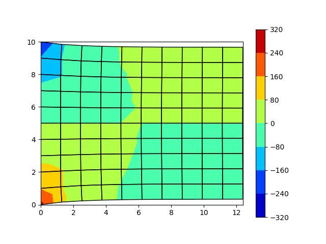
von Mises応力のプロット

コード

最後に今回用いたコードを全文張っておきます。

import numpy as np
import matplotlib.pyplot as plt
from matplotlib import patches
import matplotlib.tri as tri
class Node:
    """
    Nodeのインデックス、座標および境界条件をまとめておくクラス(2次元用)
    
    Attributes:
        id (int): Nodeのインデックス番号(重複不可)
        x, y (float): Nodeのx, y座標
    """
    def __init__(self, idx, x, y):
        self.id = idx
        self.x = x
        self.y = y
        self.bc_dist = [None, None]
        self.bc_force = [0, 0]
    
    def __str__(self):
        return 'Node {}: x {}, y {}'.format(self.id, self.x, self.y)


class Element:
    """
    4角形1次要素Elementのインデックス、要素内のNode情報および要素の厚みをまとめておくクラス
    
    Attributes:
        id (int): Elementのインデックス番号(重複不可)
        node ([int, int, int, int]): 要素内のNodeのインデックスのリスト(左下から反時計回りで指定)
        thickness (float): Elementの厚み
        xy (ndarray(size: 2, 4)): Element内のNodeのxy座標まとめ
    """
    def __init__(self, idx, node_idxs, thickness):
        self.id = idx
        self.node = node_idxs
        self.thickness = thickness
        self.xy = None

    def __str__(self):
        return 'Element {}: Nodes {}, Thickness: {}'.format(self.id, self.node, self.thickness)
    
    def get_coordination(self, nodes_dict):
        """
        要素の各節点のx,y座標を求めてself.xyに代入。

        Args:
            nodes_dict ({Node.id: Node}): Nodeの辞書
        """

        res = []
        for node_idx in self.node:
            res.append([nodes_dict[node_idx].x, nodes_dict[node_idx].y])
        self.xy = np.array(res)


class Mesh:
    """
    NodeオブジェクトとElementオブジェクトをまとめておくクラス
    
    Attributes:
        id (int): メッシュのID(重複不可)
        nodes ({Node.id: Node}): Nodeの辞書
        elements (list): Elementのリスト
    """

    def __init__(self, idx, nodes_dict, elements):
        self.id = idx
        self.nodes = nodes_dict
        self.elements = elements
        self.get_element_coord()
    
    def get_element_coord(self):
        for elm in self.elements:
            elm.get_coordination(self.nodes)


class Material:
    """
    材料特性をまとめておくクラス
    
    Attributes:
        E (float): ヤング率
        nu (float): ポアソン比
    """

    def __init__(self, E, nu):
        self.E = E
        self.nu = nu


class Solver:
    """
    有限要素法の計算を行うクラス
    
    Attributes:
        mesh (Mesh): Meshクラス
        material (Material): Materialクラス
        D (array 3x3): Dマトリクス
    """

    def __init__(self, mesh, material):
        self.mesh = mesh
        self.material = material
        self.D = self.calc_D()

    def run(self):
        self.f, self.bc_dist_dict = self.read_boundary_cond()
        self.K = self.calc_K()
        self.d = self.solve()
        self.stress_dict = self.calc_stress()

    def calc_D(self):
        """
        Dマトリクスを算出。

        Returns:
            D (array 3x3): Dマトリクス
        """
        D = np.array([[1, self.material.nu, 0],
                           [self.material.nu, 1, 0],
                           [0, 0, (1 - self.material.nu) / 2]]) \
                 * self.material.E / (1 - self.material.nu ** 2)
        return D
    
    def calc_B(self, elem, xi, eta):
        """
        Bマトリクス及びヤコビアンを算出。

        Args:
            elem (Element): 対象のElementクラス
            xi, eta (float): Bマトリクス算出用の座標

        Returns:
            B (array 3x8): Bマトリクス
            J (array 2x2): ヤコビアン
        """
        dndxi = np.array([- 1 + eta, 1 - eta, 1 + eta, - 1 - eta]) / 4
        dndeta = np.array([- 1 + xi, - 1 - xi, 1 + xi, 1 - xi]) / 4
        x = elem.xy[:, 0]
        y = elem.xy[:, 1]
        dxdxi = np.dot(dndxi, x)
        dydxi = np.dot(dndxi, y)
        dxdeta = np.dot(dndeta, x)
        dydeta = np.dot(dndeta, y)
        J = np.array([[dxdxi, dydxi], [dxdeta, dydeta]])
        B = np.zeros((3, 8))
        for i in range(4):
            Bi = np.dot(np.linalg.inv(J), np.array([dndxi[i], dndeta[i]]).T)
            B[0, 2 * i] = Bi[0]
            B[2, 2 * i + 1] = Bi[0]
            B[2, 2 * i] = Bi[1]
            B[1, 2 * i + 1] = Bi[1]
        return B, J
    
    def calc_Ke(self, elem):
        """
        Keマトリクスを算出。

        Args:
            elem (Element): 対象のElementクラス

        Returns:
            Ke (array 8x8): 要素剛性マトリクス
        """
        gps = ((-1 / np.sqrt(3), -1 / np.sqrt(3), 1, 1), 
              (1 / np.sqrt(3), -1 / np.sqrt(3), 1, 1), 
              (1 / np.sqrt(3), 1 / np.sqrt(3), 1, 1), 
              (-1 / np.sqrt(3), 1 / np.sqrt(3), 1, 1), 
              )
        
        Ke = np.zeros((8, 8))
        for xi, eta, wi, wj in gps:
            B, J = self.calc_B(elem, xi, eta)
            Ke += wi * wj * np.dot(B.T, np.dot(self.D, B)) * np.linalg.det(J) * elem.thickness

        return Ke
    
    def calc_K(self):
        """
        Kマトリクスを算出。

        Returns:
            K (array 2node_numx2node_num): 全体剛性マトリクス
        """
        K = np.zeros((len(self.mesh.nodes) * 2, len(self.mesh.nodes) * 2))
        for elem in self.mesh.elements:
            Ke = self.calc_Ke(elem)
            for i in range(4):
                for j in range(4):
                    K[2 * elem.node[i]:2 * elem.node[i]+2,
                      2 * elem.node[j]:2 * elem.node[j]+2] += Ke[2 * i:2 * i+2, 2 * j:2 * j+2]
        return K
    
    def read_boundary_cond(self):
        """
        境界条件を読み込み。

        Returns:
            f (array 2node_num): 全体荷重ベクトル
            bc_dist_dict (dict): 全体変位ベクトルのうち、変位拘束のあるindをまとめた辞書
        """
        bc_dist_dict = {}
        f = []
        for k,v in self.mesh.nodes.items():
            f += v.bc_force
            if v.bc_dist[0] is not None:
                bc_dist_dict[k * 2] = v.bc_dist[0]
            if v.bc_dist[1] is not None:
                bc_dist_dict[k * 2 + 1] = v.bc_dist[1]
        return np.array(f), bc_dist_dict
    
    def solve(self):
        for i in range(len(self.mesh.nodes) * 2):
            if i in self.bc_dist_dict.keys():
                self.K[i, :] = np.zeros(len(self.mesh.nodes) * 2)
                self.K[:, i] = np.zeros(len(self.mesh.nodes) * 2)
                self.K[i, i] = 1.0
        d = np.dot(np.linalg.inv(self.K), self.f.T)
        return d
    
    def plot_deform(self, ratio=50):
        x = np.array([[node.x, node.y] for idx, node in self.mesh.nodes.items()])
        x_new = x + self.d.reshape(len(self.mesh.nodes), 2) * ratio
        fig, ax = plt.subplots()
        for v in self.mesh.elements:
            patch = patches.Polygon(xy=v.xy, ec='black', alpha=0.3, fill=False)
            ax.add_patch(patch)
        for v in self.mesh.elements:
            xy_new = [(x_new[idx, 0], x_new[idx, 1]) for idx in v.node]
            patch = patches.Polygon(xy=xy_new, fc='red', ec='red', alpha=0.3, fill=False)
            ax.add_patch(patch)
        ax.autoscale()
        ax.set_aspect('equal', 'box')
        plt.show()
    
    def calc_stress(self):
        """
        節点応力を算出。

        Args:
            elem (Element): 対象のElementクラス

        Returns:
            stress_e (array 3x1): 節点応力
        """
        stress_dict = {i : np.zeros(3) for i in range(len(self.mesh.nodes))}
        counts_dict = {i : 0 for i in range(len(self.mesh.nodes))}

        gps = ((-1 / np.sqrt(3), -1 / np.sqrt(3), 1, 1), 
              (1 / np.sqrt(3), -1 / np.sqrt(3), 1, 1), 
              (1 / np.sqrt(3), 1 / np.sqrt(3), 1, 1), 
              (-1 / np.sqrt(3), 1 / np.sqrt(3), 1, 1), 
              )
        
        for elem in self.mesh.elements:
            nodes_ind = []
            for ind in elem.node:
                nodes_ind.append(ind * 2)
                nodes_ind.append(ind * 2 + 1)
                d_elem = self.d[nodes_ind]

            stress_e = {}
            ave_stress_e = np.zeros(3)
            for i, gp in enumerate(gps):
                xi, eta = gp[0], gp[1]
                B, J = self.calc_B(elem, xi, eta)
                stress_e[i] = np.dot(self.D, np.dot(B, d_elem).T)
                ave_stress_e += stress_e[i]
            ave_stress_e /= 4

            for i in range(4):
                stress_dict[elem.node[i]] += (stress_e[i] - ave_stress_e) * np.sqrt(3) \
                                            + ave_stress_e
                counts_dict[elem.node[i]] += 1

        for i in range(len(self.mesh.nodes)):
            stress_dict[i] = stress_dict[i] / counts_dict[i]
            res = stress_dict[i]
            misses = np.sqrt((res[0]-res[1])**2 + res[0]**2 + res[1]**2 + 6*res[2]**2)/np.sqrt(2)
            stress_dict[i] = np.append(stress_dict[i], misses)
        return stress_dict
    
    def plot_stress(self, stress_idx=0, ratio=50):
        """
        応力プロットを作成。

        Args:
            stress_idx (int(0~3)): 0-x応力, 1-y応力, 2-せん断応力, 3-von Mises
            ratio (float): 変形の倍率
        """
        x = np.array([[node.x, node.y] for idx, node in self.mesh.nodes.items()])
        x_new = x + self.d.reshape(len(self.mesh.nodes), 2) * ratio
        nodal_values = []
        for i in range(len(self.mesh.nodes)):
            nodal_values.append(self.stress_dict[i][stress_idx])

        nodes_x = x_new[:, 0]
        nodes_y = x_new[:, 1]
        elements_tris = []
        for v in self.mesh.elements:
            elements_tris.append([v.node[0], v.node[1], v.node[2]])
            elements_tris.append([v.node[0], v.node[2], v.node[3]])
        triangulation = tri.Triangulation(nodes_x, nodes_y, elements_tris)
        fig, ax = plt.subplots()
        result = ax.tricontourf(triangulation, nodal_values, cmap='jet')
        for v in self.mesh.elements:
            xy_new = [(x_new[idx, 0], x_new[idx, 1]) for idx in v.node]
            patch = patches.Polygon(xy=xy_new,ec='black', fill=False)
            ax.add_patch(patch)
        ax.autoscale()
        ax.set_aspect('equal', 'box')
        fig.colorbar(result, ax=ax)
        plt.show()

def create_mesh(length, height, mesh_size, thickness):
    """
    モデルを格子点に分割し、全ての点のNodeクラスおよびそれらを使用した4角形1次要素を作成する.
    ただし、モデル形状は四角形とする。
    
    Args:
        length, height (float): モデルの長さ、高さ
        mesh_size (float): 分割したいメッシュのサイズ
        thickness (float): 要素の厚み(今回は全て一定とする)
        
    Returns:
        nodes_dict ({Node.id: Node}): 作成したNodeの辞書
        elsms (list): 作成したElementクラスをまとめたリスト
    """
    # Nodeの作成
    num_mesh_len = int(length / mesh_size)
    num_mesh_hei = int(height / mesh_size)
    if num_mesh_len == 0:
        num_mesh_len = 1
    if num_mesh_hei == 0:
        num_mesh_hei = 1
    x = np.linspace(0, length, num_mesh_len + 1)
    y = np.linspace(0, height, num_mesh_hei + 1)
    X, Y = np.meshgrid(x, y)
    X = X.ravel()
    Y = Y.ravel()

    nodes_dict = {}
    for i, coord in enumerate(zip(X, Y)):
        nodes_dict[i] = Node(i, coord[0], coord[1])
    
    # Elementの作成
    node_idx = 0
    elem_idx = 0
    elems = []
    for i in range(num_mesh_hei):
        for j in range(num_mesh_len + 1):
            if (node_idx + 1) % (num_mesh_len + 1) == 0:
                node_idx += 1
                continue
            else:
                node_idxs = [node_idx, node_idx + 1,
                         node_idx + num_mesh_len + 2, node_idx + num_mesh_len + 1]
                elems.append(Element(elem_idx, node_idxs, thickness))
                node_idx += 1
                elem_idx += 1
    return nodes_dict, elems


def plot_mesh(mesh):
    fig, ax = plt.subplots()
    for elem in mesh.elements:
        patch = patches.Polygon(xy=elem.xy, ec='black')
        ax.add_patch(patch)
        text_xy = np.mean(elem.xy, axis=0)
        ax.text(text_xy[0], text_xy[1], elem.id, fontsize=12, va='center', ha='center')
    for node in mesh.nodes.values():
        ax.scatter(node.x, node.y, fc='black', s=100)
        ax.text(node.x, node.y, node.id, fontsize=8, color='white', va='center', ha='center')
    ax.autoscale()
    ax.set_aspect('equal', 'box')
    plt.show()


MESH_SIZE = 1
LENGTH = 10.
HEIGHT = 10.
THICKNESS = 1.
E = 208000 # ヤング率
NU = 0.27 # ポアソン比

nodes_dict, elems = create_mesh(LENGTH, HEIGHT, MESH_SIZE, THICKNESS)
mesh = Mesh(0, nodes_dict, elems)
material = Material(E, NU)

num_mesh_len = int(LENGTH / MESH_SIZE)
num_mesh_hei = int(HEIGHT / MESH_SIZE)
if num_mesh_len == 0:
    num_mesh_len = 1
if num_mesh_hei == 0:
    num_mesh_hei = 1

for k, v in mesh.nodes.items():
    # x変位の境界条件を設定
    if v.x == 0.0:
        v.bc_dist[0] = 0.0
    # y変位の境界条件を設定
    if v.x == 0.0:
        v.bc_dist[1] = 0.0
    # 荷重の設定
    if v.x == LENGTH and (v.y == 0.0 or v.y == HEIGHT):
        v.bc_force = [10000 / num_mesh_hei / 2, 0.0]
    elif v.x == LENGTH:
        v.bc_force = [10000 / num_mesh_hei, 0.0]

solver = Solver(mesh, material)
solver.run()
solver.plot_deform()
solver.plot_stress(0, 50)
solver.plot_stress(1, 50)
solver.plot_stress(2, 50)
solver.plot_stress(3, 50)